State-Adaptive Neuro-Fuzzy Inference System S-ANFIS

The State-Adaptive Neuro-Fuzzy Inference System (S-ANFIS) is a simple generalization of the ANFIS network that provides a more flexible framework for modeling complex systems by distinguishing between state variables and explanatory variables.

Core Concept of S-ANFIS

The key innovation of S-ANFIS lies in dividing input variables into two categories:

• State Variables ($s$): Used to determine the current macroscopic state or operating mode of the system
• Explanatory Variables ($x$): Variables that explain or predict system behavior within a specific state

This distinction allows the model to adopt different parameter configurations in different states, thereby better adapting to state-dependent behavioral patterns in complex systems.

S-ANFIS Network Structure and Mathematical Representation

S-ANFIS employs a two-stage neuro-fuzzy modeling approach:

Premise Part: State Identification and Association Degree Calculation

In the premise part, S-ANFIS only processes state variables $s$, aiming to identify the current system state and calculate the matching degree with each predefined state.

Assuming there are $N_s$ state variables, each with $M$ fuzzy membership functions, there will be a total of $M^{N_s}$ fuzzy rules. The total number of premise parameters is $M^{N_s} \times K$, where $K$ is the number of trainable parameters for each membership function.

For each state variable $s_j$, the membership degree after fuzzification is: \(\begin{equation} \mu_{j,m}(s_j) = \text{MF}_{j,m}(s_j; \theta_p) \end{equation}\)

where $\text{MF}_{j,m}$ represents the $m$-th membership function of the $j$-th state variable, and $\theta_p$ is the set of premise parameters.

The rule firing strength is calculated using a T-norm (such as product): \(\begin{equation} w_i = \prod_{j=1}^{N_s} \mu_{j,m_j}(s_j) \end{equation}\)

where $i$ is the rule number, and $m_j$ represents the membership function index of the $j$-th state variable corresponding to that rule.

Consequent Part: Explanatory Variable Weighting and Output

In the consequent part, S-ANFIS processes explanatory variables $x$ for each state (rule), establishing corresponding sub-models.

For the $i$-th rule, the consequent part is typically a linear combination of explanatory variables: \(\begin{equation} f_i(x) = p_{i0} + p_{i1}x_1 + p_{i2}x_2 + ... + p_{iN_x}x_{N_x} \end{equation}\)

where $p_{ij}$ are the consequent parameters to be optimized, and $N_x$ is the number of explanatory variables. The total number of consequent parameters is $M^{N_s} \times (N_x+1)$.

Final Output: Weighted Model Combination

The final output of S-ANFIS is the weighted average of the outputs from all rules: \(\begin{equation} O = \frac{\sum_{i=1}^{M^{N_s}} w_i f_i(x)}{\sum_{i=1}^{M^{N_s}} w_i} \end{equation}\)

This structure enables the model to adaptively switch between different sub-models based on the values of state variables, achieving more accurate predictions.

S-ANFIS Network Example

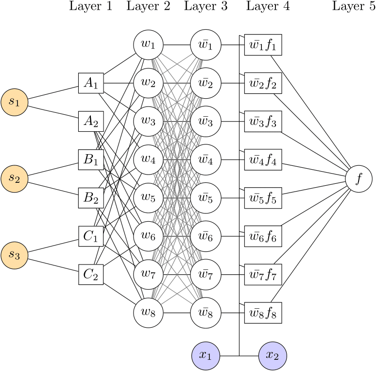
As shown in the figure above, for an S-ANFIS network with $N_s=3$ state variables and $M=2$ membership functions per variable:

• Number of rules: $M^{N_s} = 2^3 = 8$ rules
• Number of premise parameters: $M^{N_s} \times K$, depending on the membership function type
• Number of consequent parameters: $M^{N_s} \times (N_x+1) = 8 \times 3 = 24$, indicating $N_x = 2$, i.e., there are 2 explanatory variables

This network structure divides the input space into 8 fuzzy subspaces, each with its own parameter configuration.

Implementation Details

Initialization

In S-ANFIS implementation, premise parameters are typically initialized at equal intervals within the workspace to ensure sufficient overlap of membership functions. Three types of membership functions are currently supported:

1. Generalized Bell Function: \(\mu(x) = \frac{1}{1 + \left\lvert\frac{x-c}{a}\right\rvert^{2b}}\)
2. Gaussian Function: $\mu(x) = e^{-\frac{(x-c)^2}{2\sigma^2}}$
3. Sigmoid Function: $\mu(x) = \frac{1}{1 + e^{-\gamma(x-c)}}$

Consequent parameters are randomly initialized with uniform distribution in the range of $[-0.5, 0.5]$.

Feature Scaling

Input data is standardized before fitting the model: \(\begin{equation} \tilde{x}_n = \frac{x_n - \mu_{x,train}}{\sigma_{x,train}} \quad \text{and} \quad \tilde{s}_n = \frac{s_n - \mu_{s,train}}{\sigma_{s,train}} \end{equation}\)

Loss Function and Optimization

S-ANFIS uses Mean Squared Error (MSE) as the loss function: \(\begin{equation} L(\theta) = MSE = \frac{1}{N}\sum_{n=1}^{N}(O_n - \tilde{y}_n)^2 \end{equation}\)

Optimization employs the ADAM algorithm combined with elitist principles to avoid local optima: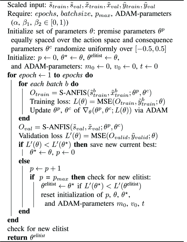

Data is divided into training and validation samples. \(\theta\) represents the set of model weights \(\theta^p\) (premise parameters) and \(\theta^c\) (consequent parameters), which are initialized differently. Model weight updates are based on the training loss function \(\operatorname{MSE}\left(O_{\text {train }}, \tilde{y}_{\text {train }}^b\right)\), where \(b\) represents the batch. To prevent overfitting and achieve regularization, an early stopping mechanism is employed: whenever the validation sample error \(L^{\prime}(\theta)\) improves, a copy of the current model parameters \(\theta^*\) is saved. $p$ is used to record the number of consecutive deteriorations in the out-of-sample loss \(L\left(O_{v a l}, y_{v a l}^b\right)\). The patience threshold \(p_{\max }\) specifies the maximum number of consecutive deteriorations allowed. When \(p\) reaches \(p_{\max }\), the system compares the current model weights with the current optimal solution, replacing it if the new solution is better in terms of out-of-sample loss. Afterwards, all optimization parameters and model weights \(\theta\) are reset, and iteration begins again in the next training cycle. The number of parameter updates depends on the number of training cycles and batch size, thus affecting computational resources—halving the batch size doubles the number of model weight updates.

S-ANFIS Advantages and Applications

S-ANFIS has several significant advantages:

1. State-Aware Modeling: Able to identify and adapt to different operating states of the system, providing specialized sub-models for each state
2. Retains ANFIS Benefits: Inherits ANFIS’s ability to transform expert knowledge, parameter training framework, and interpretability
3. Flexible Model Architecture: Can set state variables and explanatory variables according to needs, even allowing them to overlap
4. State Recognition Capability: The premise part itself can be used to study dynamic interactions between state variables and identify different operating modes of the system

This model is particularly suitable for complex systems with multiple operating states or modes, such as:

• Industrial control systems with mode switching
• Time series prediction influenced by external factors
• Nonlinear dynamic system modeling

Implementation Example

S-ANFIS can be implemented using PyTorch. Here is a simple usage example:

import numpy as np
import torch
from sanfis import SANFIS, plottingtools
from sanfis.datagenerators import sanfis_generator

# Set random seed
np.random.seed(3)
torch.manual_seed(3)

# Generate data
S, S_train, S_valid, X, X_train, X_valid, y, y_train, y_valid = sanfis_generator.gen_data_ts(
  n_obs=1000, test_size=0.33, plot_dgp=True)

# Define membership functions
membfuncs = [
  {'function': 'sigmoid',
   'n_memb': 2,
   'params': {'c': {'value': [0.0, 0.0],
            'trainable': True},
        'gamma': {'value': [-2.5, 2.5],
              'trainable': True}}},

  {'function': 'sigmoid',
   'n_memb': 2,
   'params': {'c': {'value': [0.0, 0.0],
            'trainable': True},
        'gamma': {'value': [-2.5, 2.5],
              'trainable': True}}}
]

# Create model
fis = SANFIS(membfuncs=membfuncs, n_input=2, scale='Std')
loss_function = torch.nn.MSELoss(reduction='mean')
optimizer = torch.optim.Adam(fis.parameters(), lr=0.005)

# Train model
history = fis.fit([S_train, X_train, y_train], [S_valid, X_valid, y_valid],
          optimizer, loss_function, epochs=1000)

# Evaluate model
y_pred = fis.predict([S, X])
plottingtools.plt_prediction(y, y_pred)

Conclusion

S-ANFIS provides a flexible and powerful framework for modeling complex systems by distinguishing between state variables and explanatory variables. It not only adapts to different operating states of the system but also retains the advantages of traditional ANFIS, including expert knowledge transformation, parameter training, and interpretability. This model is particularly effective when dealing with systems that have multiple operating modes or state-dependent behaviors.