Sobol Sequence - Quasi-Random Sequence Generator and Its Python Implementation

Random numbers play a crucial role in many fields including cryptography, computer graphics, and statistics. Different applications require different types of random numbers, leading to various types of random number generation. The Sobol sequence is a special type of sequence in the category of quasi-random numbers, widely used in many fields due to its excellent uniform distribution properties.

Introduction: Importance and Classification of Random Numbers

Before diving into Sobol sequences, let’s briefly review the main types of random numbers:

• Statistically Pseudorandom Numbers: These are random number sequences that approximate true random sequences in statistical properties (such as uniformity, independence). For example, in a pseudorandom bit stream, the number of 0s and 1s should be roughly equal.
• Cryptographically Secure Pseudorandom Numbers (CSPRNG): Beyond meeting the properties of statistical pseudorandom numbers, these require that predicting any part of the sequence from other parts is computationally infeasible. This is crucial for security-related applications like key generation.
• True Random Numbers: Generated based on unpredictable physical processes (such as thermal noise, radioactive decay), making samples non-reproducible. Obtaining true random numbers typically comes at a higher cost.

These random number requirements become progressively stricter, with increasing difficulty in generation. Therefore, in practical applications, we need to choose appropriate random number generation methods based on specific requirements.

Quasi-Random Number Generators (QRNG) and Low-Discrepancy Sequences

In many applications, especially Monte Carlo methods, we need points that are uniformly distributed in the sampling space. Quasi-Random Number Generators (QRNG) are designed for this purpose, generating what are known as Low-Discrepancy Sequences.

Unlike pseudorandom numbers, low-discrepancy sequences don’t aim to “look random” but rather focus on covering the sampling space more uniformly and systematically, avoiding both high clustering of points and large empty regions. Common low-discrepancy sequences include Halton sequences, Faure sequences, Niederreiter sequences, and our focus in this article—Sobol sequences.

All random number generation algorithms based on modern CPUs are typically pseudorandom, generating sequences through deterministic algorithms that repeat after a very long period. Quasi-random sequences, like Sobol sequences, are also deterministic but are designed for low discrepancy, meaning high uniformity.

Two Important Dimensions of Randomness

From an application perspective, we often need to evaluate random sequences from two dimensions:

1. Statistical Randomness: The degree of randomness in a statistical sense, such as uniformity, correlation, and repetition period. This can be assessed through various statistical tests.

2. Spatial Uniformity: The distribution characteristics of the sequence in space, especially in multi-dimensional cases. This is typically quantified using discrepancy.

For a point set $P = {\mathbf{x}_1, \dots, \mathbf{x}_N}$ in an $s$-dimensional unit hypercube $[0,1]^s$, its discrepancy $D_N(P)$ can be expressed as: \(\begin{equation} D_N(P) = \sup_{B \in J} \left| \frac{A(B; P)}{N} - \lambda_s(B) \right| \end{equation}\)

where:

• $J$ is the set of all subregions of $[0,1]^s$ with specific shapes (such as axis-aligned subrectangles).
• $A(B; P)$ is the number of points from set $P$ that fall within subregion $B$.
• $N$ is the total number of points in set $P$.
• $\lambda_s(B)$ is the $s$-dimensional volume (or measure) of subregion $B$.

Simply put, discrepancy measures the maximum deviation between the proportion of points in a subregion and the volume of that subregion in the worst case. Point sets with more uniform distribution have lower discrepancy.

Depending on the application scenario, we may focus more on one dimension. For example, statistical randomness is more important in encryption applications, while spatial uniformity may be more critical in numerical integration. Quasi-random sequences (like Sobol sequences) are specifically optimized for spatial uniformity.

What is a Sobol Sequence?

A Sobol sequence is a series of $n$-dimensional points designed to be more uniformly distributed in the unit hypercube $[0, 1)^n$ than standard pseudo-random sequences.

• Deterministic: Points in a Sobol sequence are completely determined for a given dimension and index, unlike pseudo-random numbers that depend on random seeds (although some implementations allow “scrambling” to introduce randomness while maintaining low discrepancy).
• Low Discrepancy: This is the core characteristic of Sobol sequences. Discrepancy is a measure of how uniformly points are distributed. Low discrepancy means the point set better avoids large gaps or excessive clustering of points.

The following figure intuitively shows the difference between pseudorandom point sets and low-discrepancy sequence point sets:

Left: two-dimensional point set composed of pseudorandom numbers; Right: point set from a low-discrepancy sequence (like Sobol sequence), showing more complete and uniform coverage of the space.

How are Sobol Sequences Generated?

Sobol sequences are generated based on binary arithmetic and a special set of numbers called direction numbers or initialization numbers. The core idea is related to Radical Inversion and Van der Corput sequences.

Radical Inversion and Van der Corput Sequences

Radical Inversion is a method of mapping an integer $i$ to the interval $[0,1)$. For a base $b$, an integer $i$ can be represented in base $b$ as: \(\begin{equation} i = \sum_{l=0}^{M-1} a_l(i) b^l \end{equation}\)

Its Radical Inversion $\Phi_b(i)$ (in the simplified case where $C$ is the identity matrix, i.e., Van der Corput sequence) is defined as: \(\begin{equation} \Phi_b(i) = \sum_{l=0}^{M-1} a_l(i) b^{-l-1} \end{equation}\)

This effectively mirrors the digits of $i$’s base-$b$ representation from left to right of the decimal point.

For example, the first few terms of the base-2 Van der Corput sequence:

• $i=1=(1)_2 \implies \Phi_2(1) = (0.1)_2 = 1/2$
• $i=2=(10)_2 \implies \Phi_2(2) = (0.01)_2 = 1/4$
• $i=3=(11)_2 \implies \Phi_2(3) = (0.11)_2 = 3/4$
• $i=4=(100)_2 \implies \Phi_2(4) = (0.001)_2 = 1/8$

Each point in this sequence takes the midpoint of the currently longest uncovered interval, thus ensuring uniform distribution.

Sobol Sequence Construction

Each dimension of a Sobol sequence can be viewed as a generalization of a base-2 Van der Corput sequence using different generating matrices $\mathbf{C}_j$ (corresponding to direction numbers). The $i$-th point $\boldsymbol{X}_i$ of an $n$-dimensional Sobol sequence can be expressed as: \(\begin{equation} \boldsymbol{X}_i = \left( \boldsymbol{\Phi}_{2, \mathbf{C}_1}(i), \boldsymbol{\Phi}_{2, \mathbf{C}_2}(i), \ldots, \boldsymbol{\Phi}_{2, \mathbf{C}_n}(i) \right) \end{equation}\)

where $\boldsymbol{\Phi}_{2, \mathbf{C}_j}(i)$ is the coordinate for dimension $j$, obtained through a series of bitwise XOR operations between the binary representation of integer $i$ and a set of direction numbers (encoded in $\mathbf{C}_j$) for dimension $j$.

Specifically, for the $k$-th point and dimension $j$:

1. Express $k$ in binary form: $k = (b_m b_{m-1} \dots b_1)_2$
2. The coordinate $x_{k,j}$ can be expressed as $x_{k,j} = b_1 v_{j,1} \oplus b_2 v_{j,2} \oplus \dots \oplus b_m v_{j,m}$, where $\oplus$ is the XOR operation, and $v_{j,r}$ is the $r$-th direction number for dimension $j$ (itself a binary fraction in $[0,1)$).

Being entirely base-2, Sobol sequences can be efficiently implemented using bitwise operations (like right shifts and XOR), making computation very fast. The choice of primitive polynomials and derived direction numbers is crucial for ensuring the low-discrepancy property of Sobol sequences.

A notable property is that when the number of samples $N$ is a power of 2 (e.g., $N=2^k$), the Sobol sequence will have exactly one point in each base-2 elementary interval of $[0,1)^s$. This means it can generate samples of quality comparable to Stratified Sampling or Latin Hypercube Sampling without requiring the total number of samples to be predetermined.

Advantages and Disadvantages of Sobol Sampling

Advantages:

1. Superior Uniformity: Especially in high-dimensional spaces, Sobol sequences cover the sampling space more effectively and uniformly than pseudorandom numbers.
2. Faster Convergence Rate: In numerical integration (quasi-Monte Carlo integration) for s-dimensional problems, standard Monte Carlo methods using N points typically converge at $O(N^{-1/2})$. Low-discrepancy sequences like Sobol can achieve $O(N^{-1}(\log N)^s)$ or better, meaning comparable accuracy with fewer samples.
3. Deterministic and Reproducible: When unscrambled, the sequence is deterministically generated, making results reproducible - beneficial for debugging and comparison.
4. Efficient Parameter Space Exploration: Well-suited for systematically exploring multi-dimensional parameter spaces in applications like hyperparameter optimization and sensitivity analysis.
5. Progressive Generation: Points can be generated incrementally without knowing total sample size N, with subsequences maintaining good distribution properties. Ideal for progressive sampling.

Disadvantages and Considerations:

1. Poor Initial Point Projections: For small sample sizes (e.g., much less than $2^d$, where d is dimension), Sobol sequences may show patterns or alignment in certain low-dimensional projections, appearing less “random”.
2. Direction Number Quality: Sequence quality heavily depends on direction numbers used. Some early direction number sets performed poorly in high dimensions. Modern implementations use optimized sets (e.g., Joe-Kuo direction numbers).
3. Dimensionality Limitations: While theoretically extensible to high dimensions, computing and storing quality direction numbers becomes challenging. For extremely high dimensions (thousands), advantages over standard Monte Carlo may diminish or require complex scrambling.
4. Scrambling: To mitigate poor initial projections and improve finite-sample randomness, Sobol sequences can be “scrambled” (random linear scrambling or digital shifts). This introduces randomness while maintaining low discrepancy.

Comparison between Sobol Sequences and Regular Grid Sampling (linspace)

A common question arises: since Sobol sequences aim for uniform distribution, why not simply use functions like np.linspace to create equidistant points in each dimension and combine them into a regular multidimensional grid?

While regular grids are intuitive and easy to implement for uniform coverage in low dimensions (like 1D or 2D), low-discrepancy sequences like Sobol sequences often have advantages in multidimensional spaces and many practical applications. Here’s why:

1. Curse of Dimensionality:
   • Regular Grid: For $d$ dimensions with $k$ points per dimension, the total number of points is $k^d$. As dimension $d$ increases, the required points grow exponentially, quickly becoming computationally infeasible. For example, 10 dimensions with 10 points each requires $10^{10}$ (10 billion) samples.
   • Sobol Sequence: Can flexibly generate any number $N$ of sample points that collectively work to fill the $d$-dimensional space uniformly, where $N$ is typically much smaller than $k^d$, making it more practical for high dimensions.
2. Projection Properties and “Alignment” Artifacts:
   • Regular Grid: Points are strictly aligned on grid lines, forming highly regular structures. This regularity may cause systematic bias when sampling points align with specific structures in the studied function or phenomenon.
   • Sobol Sequence: Though deterministic, it’s designed to minimize discrepancy, ensuring more uniform point distribution in various subregions (especially axis-aligned ones), avoiding rigid grid structures while maintaining good distribution in low-dimensional projections.
3. Progressive Generation Property:
   • Regular Grid: Usually requires predetermining total points and grid structure. Increasing samples often means regenerating an entirely new, denser grid, potentially unable to directly reuse existing samples.
   • Sobol Sequence: Features point-by-point generation. Can generate $N_1$ points initially, and if higher precision is needed, generate additional points to form a sequence of $N_1+N_2$ points, where the first $N_1$ points remain consistent with the original sequence while maintaining low discrepancy. This is valuable for progressive improvement and adaptive sampling.
4. Integration Convergence and Efficiency:
   • Regular Grid (for numerical integration): While some grid-based quadrature rules (like trapezoidal or Simpson’s) have good convergence order for smooth functions, they’re limited by fixed grid structure and may have poor constant factors in high dimensions.
   • Sobol Sequence (for quasi-Monte Carlo integration, QMC): QMC methods can theoretically achieve error convergence rates of $O(N^{-1}(\log N)^s)$, typically better than standard Monte Carlo’s $O(N^{-1/2})$. For medium to high dimensions, QMC is usually more flexible and efficient than deterministic quadrature rules based on fixed grids.
5. Space “Filling” Method:
   • Regular Grid: Like laying “tiles” regularly in space.
   • Sobol Sequence: More like “intelligently” placing points to ensure comprehensive coverage while avoiding gaps and clustering, without the rigidity of a grid.

Regular grids generated by linspace primarily ensure equidistance in single dimensions, while Sobol sequences aim for low discrepancy and high uniformity across the entire multidimensional space. Therefore, Sobol sequences are superior to regular grid sampling in high-dimensional problems, applications requiring progressive generation capability, or faster integration convergence. Regular grid sampling is more suitable for very low-dimensional scenarios or when strict control of sampling positions in each dimension is needed.

Main Applications of Sobol Sampling

Sobol sampling finds wide application across multiple domains:

1. Numerical Integration: The classic and primary application through quasi-Monte Carlo integration.
2. Financial Engineering: Used in derivative pricing (e.g., option pricing), Value at Risk (VaR) calculations, and credit risk models.
3. Computer Graphics: Employed in global illumination algorithms (path tracing, ray tracing sampling), anti-aliasing for smoother, more realistic images.
4. Sensitivity Analysis: Evaluating model output sensitivity to input parameter changes through efficient parameter space exploration.
5. Optimization: Used as initialization or search strategy in global optimization algorithms (particle swarm optimization or simulated annealing).
6. Physics and Engineering Simulation: Applications requiring extensive simulation and parameter studies.
7. Machine Learning: Such as exploring parameter combinations in hyperparameter optimization for finding optimal configurations.

Sobol Sequence Implementation in Python

Several Python libraries provide implementations of Sobol sequences, with SciPy and PyTorch being the most commonly used.

Using SciPy (scipy.stats.qmc.Sobol)

The stats.qmc (Quasi-Monte Carlo) module in SciPy provides the Sobol class.

# 1. Initialize Sobol sequence generator
dimension = 2  # define dimension
# Sobol sequence generator, can specify scramble=True for scrambling
sobol_engine = qmc.Sobol(d=dimension, scramble=False, seed=None) # seed for randomness when scrambling

# 2. Generate sample points
num_samples = 128
samples = sobol_engine.random(n=num_samples) # generate num_samples points

print(f"Generated {num_samples} Sobol samples of dimension {dimension}:")
print(samples[:5]) # print first 5 sample points

# 3. Skip initial points (optional)
# Sometimes we skip the initial part of the sequence for better distribution properties
# sobol_engine_skipped = qmc.Sobol(d=dimension, scramble=False)
# sobol_engine_skipped.fast_forward(1024) # skip first 1024 points
# samples_skipped = sobol_engine_skipped.random(n=num_samples)
# print("\nSobol samples after skipping 1024 points:")
# print(samples_skipped[:5])

# 4. Use scrambling
sobol_engine_scrambled = qmc.Sobol(d=dimension, scramble=True, seed=42)
samples_scrambled = sobol_engine_scrambled.random(n=num_samples)
print("\nScrambled Sobol samples:")
print(samples_scrambled[:5])

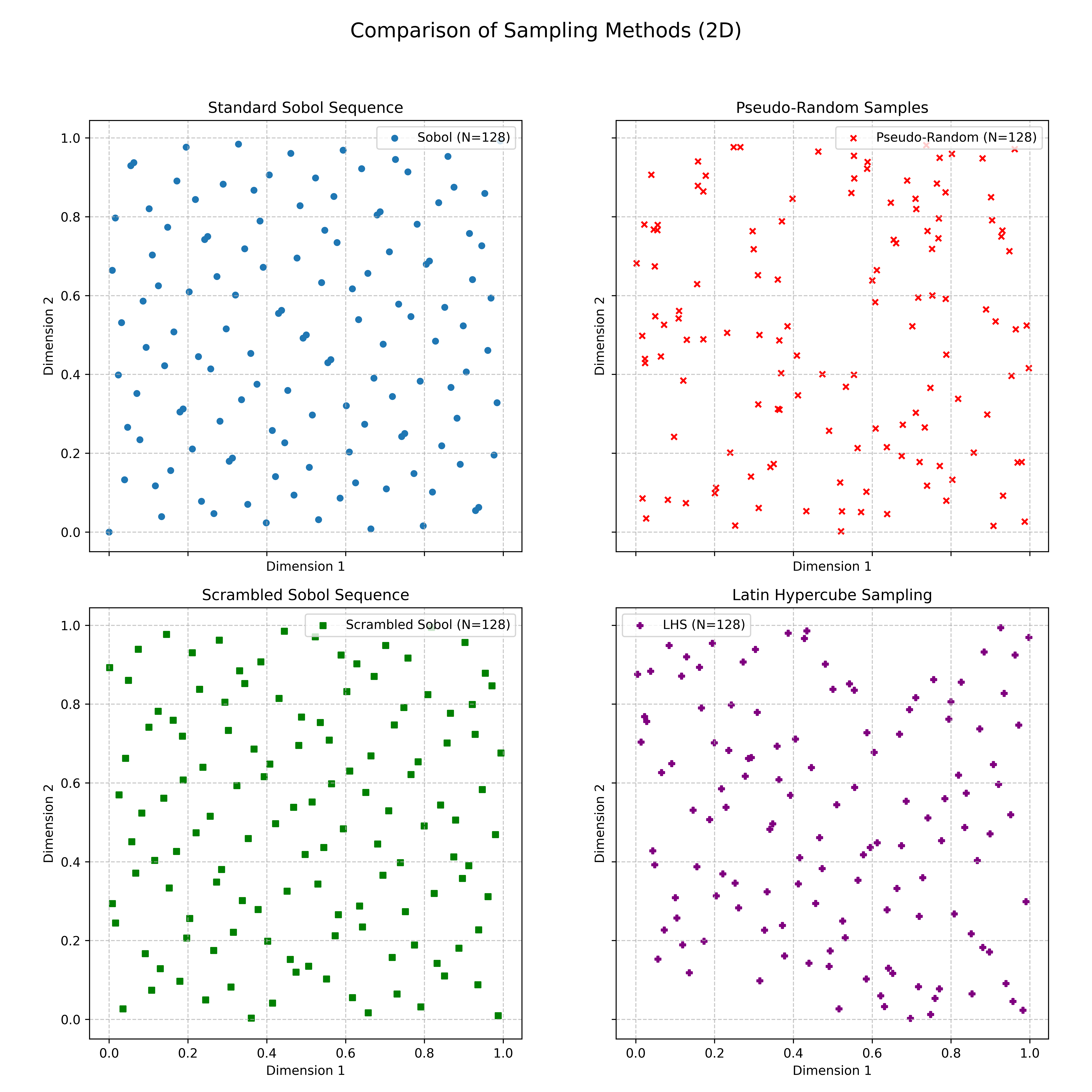
# 5. Visualization (2D only)
if dimension == 2:
    fig, axs = plt.subplots(2, 2, figsize=(12, 12), sharex=True, sharey=True)  # adjust to 2x2 layout

    # Standard Sobol sequence
    axs[0, 0].scatter(samples[:, 0], samples[:, 1], s=20, marker='o', label=f'Sobol (N={num_samples})')
    axs[0, 0].set_title('Standard Sobol Sequence')
    axs[0, 0].set_xlabel('Dimension 1')
    axs[0, 0].set_ylabel('Dimension 2')
    axs[0, 0].set_aspect('equal', adjustable='box')
    axs[0, 0].legend()
    axs[0, 0].grid(True, linestyle='--', alpha=0.7)

    # Pseudo-random numbers for comparison
    pseudo_random_samples = np.random.rand(num_samples, dimension)
    axs[0, 1].scatter(pseudo_random_samples[:, 0], pseudo_random_samples[:, 1], s=20, marker='x', color='red',
                      label=f'Pseudo-Random (N={num_samples})')
    axs[0, 1].set_title('Pseudo-Random Samples')
    axs[0, 1].set_xlabel('Dimension 1')
    axs[0, 1].set_ylabel('Dimension 2')
    axs[0, 1].set_aspect('equal', adjustable='box')
    axs[0, 1].legend()
    axs[0, 1].grid(True, linestyle='--', alpha=0.7)

    # Scrambled Sobol sequence
    axs[1, 0].scatter(samples_scrambled[:, 0], samples_scrambled[:, 1], s=20, marker='s', color='green',
                      label=f'Scrambled Sobol (N={num_samples})')
    axs[1, 0].set_title('Scrambled Sobol Sequence')
    axs[1, 0].set_xlabel('Dimension 1')
    axs[1, 0].set_ylabel('Dimension 2')
    axs[1, 0].set_aspect('equal', adjustable='box')
    axs[1, 0].legend()
    axs[1, 0].grid(True, linestyle='--', alpha=0.7)

    # Latin Hypercube Sampling (LHS)
    lhs_engine = qmc.LatinHypercube(d=dimension, seed=42)
    samples_lhs = lhs_engine.random(n=num_samples)
    axs[1, 1].scatter(samples_lhs[:, 0], samples_lhs[:, 1], s=20, marker='P', color='purple',
                      label=f'LHS (N={num_samples})')
    axs[1, 1].set_title('Latin Hypercube Sampling')
    axs[1, 1].set_xlabel('Dimension 1')
    axs[1, 1].set_ylabel('Dimension 2')
    axs[1, 1].set_aspect('equal', adjustable='box')
    axs[1, 1].legend()
    axs[1, 1].grid(True, linestyle='--', alpha=0.7)

    plt.suptitle('Comparison of Sampling Methods (2D)', fontsize=16)
    plt.tight_layout(rect=[0, 0, 1, 0.95])  # adjust layout for title
    plt.savefig('sampling_methods_2d.png', dpi=600)
    plt.show()

Notes:

• qmc.Sobol(d=dimension, scramble=False): Initializes a Sobol sequence generator. d is the dimension. scramble=True enables scrambling, which typically improves finite sample quality but loses pure determinism (scrambling itself is random, but for a fixed seed, the scrambled sequence is deterministic).
• sobol_engine.random(n=num_samples): Generates num_samples sample points. Each point is a dimension-dimensional vector with components in the interval $[0, 1)$.
• sobol_engine.fast_forward(m): Can skip the first m points in the sequence.
• seed: When scramble=True, seed controls the randomness of scrambling to ensure reproducibility.

Using PyTorch (torch.quasirandom.SobolEngine)

PyTorch also provides SobolEngine for generating Sobol sequences, which is particularly convenient when working within the PyTorch ecosystem (e.g., for hyperparameter search in deep learning models or gradient-based expectation estimation).

import torch
from torch.quasirandom import SobolEngine

# 1. Initialize SobolEngine
dimension = 2
# scramble=True enables scrambling, seed for reproducibility when scrambling
sobol_engine_torch = SobolEngine(dimension=dimension, scramble=False, seed=None)

# 2. Generate sample points
num_samples = 128
# draw method returns a Tensor
samples_torch = sobol_engine_torch.draw(num_samples) 

print(f"\nGenerated {num_samples} Sobol samples using PyTorch (dimension {dimension}):")
print(samples_torch[:5])

# 3. Use scrambling
sobol_engine_torch_scrambled = SobolEngine(dimension=dimension, scramble=True, seed=42)
samples_torch_scrambled = sobol_engine_torch_scrambled.draw(num_samples)
print("\nScrambled Sobol samples using PyTorch:")
print(samples_torch_scrambled[:5])

Notes:

• SobolEngine(dimension=dimension, scramble=False, seed=None): Initializes the engine. dimension is the dimensionality. scramble=True enables scrambling. seed fixes random number generator state when scrambling.
• sobol_engine_torch.draw(num_samples): Generates num_samples sample points, returning a PyTorch Tensor.
• PyTorch’s SobolEngine supports up to approximately 1111 dimensions (as of recent versions, please check official documentation), and uses optimized direction numbers.

Comparison of Different Sampling Methods

To better understand the characteristics of Sobol sequences, the following table summarizes its comparison with other common sampling methods:

Characteristic	Pseudo-Random Numbers (PRNG)	Grid Sampling	Latin Hypercube Sampling (LHS)	Halton/Hammersley Sequences	Sobol Sequences
Type	Pseudo-Random	Deterministic/Systematic	Stratified Random	Quasi-Random	Quasi-Random
Uniformity/Coverage	May have clusters and gaps	Regular, but inefficient in high dimensions; prone to artifacts	Ensures stratified uniformity in 1D projections	Good, but low-dim projections may be inferior to Sobol	Excellent, especially in high dimensions
Discrepancy	High	Low (but fixed structure)	Medium to Low	Low	Very Low
Convergence Rate (Integration)	$O(N^{-1/2})$	Depends on function, may be poor	Usually better than PRNG, near $O(N^{-1})$ (varies)	$O(N^{-1}(\log N)^s)$ or better	$O(N^{-1}(\log N)^s)$ or better
Deterministic	No (seed-dependent)	Yes	No (random within strata)	Yes	Yes (without scrambling)
Progressive Generation	Yes	Usually No (needs predefined total points)	Usually No (needs predefined total points)	Yes	Yes
Computational Cost (Generation)	Very Low	Low	Low to Medium	Low	Low (bit operations)
Correlation/Patterns	Low (theoretically), but finite period	Strong regularity, axis-aligned patterns	Avoids 1D clustering, but may have structure in high-dim	May have linear correlation for some bases	Initial projections may be poor (improvable through scrambling)
Main Advantages	Simple implementation, fast	Simple and intuitive	Guarantees good 1D coverage, effective for certain models	Good uniformity, deterministic	Excellent uniformity, fast convergence, progressive
Main Disadvantages	Slow convergence, poor high-dim coverage	“Curse of dimensionality”, inflexible	May be inferior to QMC in high-dim, non-progressive	Initial point issues, base-sensitive	Initial point issues, direction number dependent
Typical Uses	General simulation, games, cryptography (CSPRNG)	Low-dim parameter sweeps, visualization	Computer experiments, uncertainty quantification, optimization	Numerical integration, parameter space exploration	Numerical integration, finance, graphics, sensitivity analysis
Python Examples	numpy.random.rand() torch.rand()	numpy.meshgrid() itertools.product()	scipy.stats.qmc.LatinHypercube	scipy.stats.qmc.Halton	scipy.stats.qmc.Sobol torch.quasirandom.SobolEngine

Some Explanations:

• Grid Sampling: Takes equidistant points in each dimension and combines them. While intuitive in low dimensions, point requirements grow exponentially with dimensions (curse of dimensionality).
• Stratified Sampling: Divides space into non-overlapping subregions (strata) with independent sampling within each. LHS is a special form of stratified sampling.
• Latin Hypercube Sampling (LHS): Divides each dimension into N equal-probability intervals, randomly samples one value from each interval, ensuring one sample per stratum in each dimension, then randomly combines these values. Guarantees uniformity in one-dimensional projections.
• Halton/Hammersley Sequences: Classical low-discrepancy sequences. Halton uses Van der Corput sequences with different prime bases, while Hammersley modifies the first dimension.

Sobol sequences are often considered one of the best low-discrepancy sequences, particularly for high-dimensional uniform sampling and fast convergence in quasi-Monte Carlo integration.

Summary

Sobol sequences, as a classic low-discrepancy sequence, demonstrate excellent performance in multi-dimensional sampling through their deterministic generation method and superior uniform distribution properties. They can fill sampling spaces more effectively than traditional pseudorandom numbers, thereby improving computational efficiency and result accuracy in numerical integration, financial modeling, computer graphics, and machine learning applications.

Despite certain challenges such as initial point distribution and dimensional limitations, Sobol sequences remain a powerful and valuable tool in scientific computing and engineering practice, thanks to optimized direction numbers and scrambling techniques in modern implementations. Libraries like SciPy and PyTorch in Python make Sobol sequences easily accessible and usable.