Performance metrics for multi-objective optimization
In multi-objective optimization, since the solution is usually not a single one but a Pareto-optimal set of solutions (or an approximation thereof), we need suitable performance metrics to evaluate the quality of the solution set found by the algorithm.
In multi-objective optimization, since the solutions are typically not unique but form a Pareto optimal set (or its approximation), we require appropriate performance metrics to evaluate the quality of solution sets obtained by algorithms. These metrics primarily focus on two aspects:
- Convergence: The solutions should be as close as possible to the true Pareto front.
- Diversity/Spread: The solutions should be distributed as widely and uniformly as possible across the Pareto front to represent diverse trade-off options.
Hypervolume (HV) and Its Variants
Hypervolume (HV):
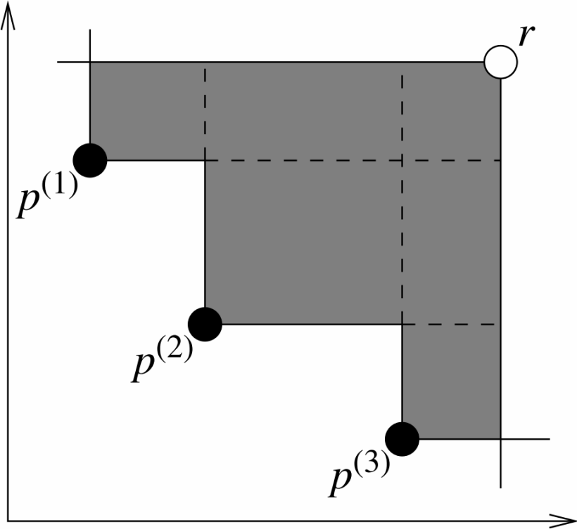
Hypervolume metric for a two-objective problem
Definition: The hypervolume metric measures the “volume” (or area in 2D) enclosed between the solution set and a predefined reference point in the objective space. The reference point is typically chosen to be “worse” than all solutions in the set (e.g., for minimization problems, each component of the reference point is larger than the maximum value of the corresponding objective in the solution set). A larger HV value generally indicates better overall performance of the solution set, as it implies better convergence to the true Pareto front and/or better diversity.
Calculation Steps:
- Determine Reference Point: The reference point is usually a point worse than all solutions in the set. For a minimization problem, each coordinate of the reference point can be the maximum value of the corresponding objective plus a large offset. For $k$ minimization objectives, the reference point $R=(r_1,r_2,…,r_k)$ should satisfy $s_i < r_i$ (strictly, $s_i \leq r_i$ for computation) for all $i=1,…,k$ and any solution $s=(s_1,…,s_k)$ in the solution set $S$.
- Compute Contribution Volume:For each non-dominated solution in $S$, compute the hyperrectangular region formed with the reference point, excluding regions dominated by other solutions.
- Sum Non-overlapping Volumes:Sum the non-overlapping hyperrectangular volumes contributed by all non-dominated solutions to obtain the total hypervolume.
A more rigorous definition based on the Lebesgue measure: \(\begin{equation} H V(\mathcal{S}, \mathbf{R})=\lambda\left(\bigcup_{\mathbf{s} \in \mathcal{S}} ⟦𝐬, 𝐑⟧\right) \end{equation}\) where ⟦𝐬, 𝐑⟧ denotes the hyperrectangle bounded by s and R, and $\lambda$ is the Lebesgue measure.
Advantages:
- Strict Pareto compliance: If solution set $A$ Pareto-dominates set $B$, then $HV(A) \geq HV(B)$.
- Simultaneously measures convergence and diversity.
- Does not require knowledge of the true Pareto front.
Disadvantages:
- High computational complexity, especially in high-dimensional objective spaces ($k > 3$).
- Sensitivity to the choice of reference point.
- Sensitivity to objective scaling; normalization of objectives is often required.
Code Implementation:
1
2
3
4
5
6
7
8
9
10
11
12
13
14
15
16
17
18
19
20
21
22
23
24
25
26
27
28
29
30
31
32
33
34
35
36
37
38
def calculate_hv_2d_min(solution_set, reference_point):
    """
    Calculate hypervolume for 2D minimization problems.
    solution_set: (n_solutions, 2) array, each row is a solution's objective values.
    reference_point: (2,) array, reference point.
    """
    solutions = np.array(solution_set)
    ref_point = np.array(reference_point)

    # Filter solutions dominated by the reference point
    valid_solutions = []
    for s in solutions:
        if np.all(s < ref_point):  # For minimization
            valid_solutions.append(s)
    if not valid_solutions:
        return 0.0

    solutions = np.array(valid_solutions)

    # Sort by first objective (ascending), then second objective (ascending)
    sorted_indices = np.lexsort((solutions[:, 1], solutions[:, 0]))
    sorted_solutions = solutions[sorted_indices]

    hv = 0.0
    previous_y = ref_point[1]  # Start from the "worst" y-value

    for i in range(sorted_solutions.shape[0]):
        width = ref_point[0] - sorted_solutions[i, 0]
        height = previous_y - sorted_solutions[i, 1]

        if width > 0 and height > 0:
            hv += width * height

        previous_y = sorted_solutions[i, 1]

        if sorted_solutions[i, 0] >= ref_point[0]:
            break
    return hv
Pymoo Implementation:
1
2
3
4
5
6
7
8
9
10
11
12
from pymoo.indicators.hv import HV
import numpy as np

# F: (n_solutions, n_objectives) array of objective values
# F = np.array([[1, 5], [2, 3], [3, 4], [4, 1]])  # Example (minimization)

# Reference point for minimization (worse than all solutions)
# ref_point = np.array([6.0, 7.0])

ind = HV(ref_point=ref_point)
hv_value = ind(F)
print(f"Hypervolume (Pymoo): {hv_value}")
Mean Hypervolume (MHV):
MHV typically refers to the average hypervolume (HV) value obtained from multiple independent runs of the same multi-objective optimization algorithm. It is used to evaluate the stability and average performance of the algorithm. \(\begin{equation} M H V=\frac{1}{N_{\text {runs }}} \sum_{i=1}^{N_{\text {runs }}} H V_i \end{equation}\)
Here, $N_{\text {runs }}$ is the number of algorithm runs, and $HV_i$ is the hypervolume of the solution set obtained in the $i$-th run.
Advantages: It reflects the average performance of the algorithm, reducing the impact of randomness from a single run.
Disadvantages: It requires multiple runs of the algorithm, which can be computationally expensive.
Hypervolume Difference (HVD):
HVD typically refers to the difference between the hypervolume of the true Pareto front (if known) and the hypervolume of the solution set found by the algorithm. \(\begin{equation} H V D=H V\left(P F_{\text {true }}\right)-H V\left(P F_{\text {approx }}\right) \end{equation}\)
Here, $PF_{\text {true }}$ is the true Pareto front, and $PF_{\text {approx}}$ is the approximate Pareto front found by the algorithm. A smaller $HVD$ is better. If $PF_{\text {true }}$ is unknown, a high-quality reference front is sometimes used instead. Another form is the relative hypervolume difference, also known as the insufficient hypervolume ratio: $1-H V\left(PF_{\text {approx }}\right) / H V\left(P F_{\text {true }}\right)$.
Generational Distance (GD) and Its Variants
Generational Distance (GD):
GD measures the average minimum distance from each solution in the approximated Pareto front $PF_{\text {approx}}$ to the true Pareto front $PF_{\text {true }}$. It primarily evaluates the convergence of the solution set. A smaller GD value indicates that the solution set is closer to the true Pareto front.
Calculation steps:
- Determine the true Pareto front $PF_{\text {true }}$: This is a set of known optimal solutions.
- Determine the computed solution set $PF_{\text {approx}}$: This is the set of solutions found by the algorithm.
- Calculate the minimum Euclidean distance between each solution and the true Pareto front: For each solution in $PF_{\text {approx}}$, calculate its Euclidean distance to all solutions $z_j$ on $PF_{\text {true }}$, and take the minimum value $d_i = \min_{z_j \in PF_{\text{true}}} \operatorname{distance}\left(x_i, z_j\right)$.
- Calculate the average of all distances:
Typically $p=2$ (root mean square of Euclidean distances), simplifying to: \(GD = \frac{1}{|PF_{approx}|} \sum_{i=1}^{|PF_{approx}|} \min_{\mathbf{z} \in PF_{true}} \sqrt{\sum_{k=1}^M (f_k(\mathbf{x}_i) - f_k(\mathbf{z}))^2}\) where $M$ is the number of objectives, $f_k(\mathbf{x}_i)$ and $f_k(\mathbf{z})$ are the values of solution $\mathbf{x}_i$ and $\mathbf{z}$ on the $k$-th objective, respectively.
Advantages:
- Intuitive, easy to understand and calculate.
- Effectively measures the convergence of the solution set.
Disadvantages:
- Requires the true Pareto front, which is unknown in many practical problems.
- If the approximate solution set has only a few points that are very close to a small region of the true front, GD value may be small, but this does not reflect the diversity of solutions.
- Sensitive to the number and distribution of points in $PF_{\text {true }}$.
Code implementation:
1
2
3
4
5
6
7
8
9
10
11
12
13
14
15
16
17
18
19
20
21
22
23
24
25
26
27
28
29
30
31
32
33
34
35
36
37
38
def calculate_gd(solution_set, reference_set):
    """
    Calculate Generational Distance (GD).
    solution_set: (n_solutions, n_objectives) array, solutions found by algorithm.
    reference_set: (n_ref_points, n_objectives) array, true Pareto front.
    """
    solution_set = np.array(solution_set)
    reference_set = np.array(reference_set)

    sum_min_distances_sq = 0.0
    for sol_point in solution_set:
        # Calculate squared Euclidean distances from current solution to all true front points
        distances_sq = np.sum((reference_set - sol_point)**2, axis=1)
        min_distance_sq = np.min(distances_sq)
        sum_min_distances_sq += min_distance_sq # Or directly add min_distance, then divide by N and sqrt at end

    # GD is usually mean or RMS of distances, here we use sqrt of mean squared distance
    # Or directly use mean of distances (p=1)
    # gd_value = np.sqrt(sum_min_distances_sq / solution_set.shape[0]) # p=2

    # More common GD is direct average of minimum distances (p=1 in the sum, then average)
    # Pymoo's GD is (sum d_i^p / N)^(1/p)
    # If p=1, then (sum d_i / N)
    # If p=2, then (sum d_i^2 / N)^(1/2)

    # To be consistent with Pymoo's GD(p=1) definition:
    accum_dist = 0
    for s_point in solution_set:
        dist = np.min(np.sqrt(np.sum((reference_set - s_point)**2, axis=1)))
        accum_dist += dist
    gd_value = accum_dist / solution_set.shape[0]
    return gd_value

# solutions = np.array([[1.1, 4.9], [2.2, 2.8]])
# pf_true = np.array([[1, 5], [2, 3], [3,4], [4,1]])
# gd_val = calculate_gd(solutions, pf_true)
# print(f"GD: {gd_val}")
Pymoo implementation:
1
2
3
4
5
6
7
8
9
10
11
12
13
14
15
from pymoo.indicators.gd import GD
import numpy as np

# F = np.array([[1.1, 4.9], [2.2, 2.8]]) # Solutions found by algorithm
# pf_true = np.array([[1, 5], [2, 3], [3,4], [4,1]]) # True Pareto front

# Initialize GD indicator calculator, pf_true is the true front
# ind = GD(pf_true, norm=False) # norm=False uses Euclidean distance, Pymoo's GD default p=1
                             # Pymoo's GD.py defined as (1/n * sum(d_i^p))^(1/p)
                             # d_i = min_{z in PF_true} ||f(x_i) - f(z)||_p_dist
                             # Default p_dist = 2 (Euclidean), p = 1 (for aggregation)

# Calculate GD value
# gd_value = ind(F)
# print(f"GD (Pymoo): {gd_value}")
GD+
GD+ (Generational Distance Plus) is a variant of GD that considers dominance relationships when calculating distances. For a solution $x$ in $PF_{\text {approx}}$, if it is dominated by some solution $z$ in $PF_{\text {true }}$, their distance is the “correction distance” needed to move from $x$ to $z$ (usually the sum of objective component differences, considering only where $x$ is worse than $z$). If $x$ is not dominated by any solution in $PF_{\text {true }}$ (i.e., $x$ is above or outside the true front), its distance is 0. A smaller GD+ value is better.
\(\begin{equation} d^{+}\left(x, P F_{\text {true }}\right)= \begin{cases}\sqrt{\sum_{k=1}^M\left(\max \left\{0, f_k(x)-f_k\left(z_x^*\right)\right\}\right)^2} & \text { if } x \text { is dominated by some } z \in P F_{\text {true }} \\ 0 & \text { otherwise }\end{cases} \end{equation}\) where $z_x^*$ is the point in $PF_{true}$ that “most closely dominates” $x$ (or a reference point that can dominate $x$). More precisely, it is based on the “dominance distance penalty”. \(\begin{equation} G D^{+}\left(P F_{\text {approx }}, P F_{\text {true }}\right)=\frac{1}{\left|P F_{\text {approx }}\right|} \sum_{x \in P F_{\text {approx }}} d^{+}\left(x, P F_{\text {true }}\right) \end{equation}\)
Advantages include better reflection than GD of whether solutions are truly “inferior” (i.e., dominated). No distance penalty is given for solutions that have already reached or surpassed the true front. However, it still requires the true Pareto front, and computation may be slightly more complex than GD.
Pymoo implementation:
1
2
3
4
5
6
7
8
9
10
from pymoo.indicators.gd_plus import GDPlus # or write as GDPlus
import numpy as np

# F = np.array([[1.1, 4.9], [2.2, 2.8], [0.5, 6.0]]) # Solutions found by algorithm
# pf_true = np.array([[1, 5], [2, 3], [3,4], [4,1]]) # True Pareto front

# ind = GDPlus(pf_true, norm=False) # Default p=1
# gd_plus_value = ind(F)
# print(f"GD+ (Pymoo): {gd_plus_value}")
Inverted Generational Distance (IGD)
IGD measures the average minimum distance from each point in the true Pareto front $PF_{\text {true }}$ to the approximated Pareto front $PF_{\text {approx}}$ found by the algorithm. IGD can evaluate both convergence and diversity of the solution set (provided that points on $PF_{\text {true }}$ are well-distributed and representative). A smaller IGD value indicates a better solution set.
Calculation steps:
- Determine the true Pareto front $PF_{\text {true }}$
- Determine the computed solution set $PF_{\text {approx}}$
- Calculate the minimum distance between each true Pareto front solution and the computed solution set: For each point $z_j$ in $PF_{\text {true }}$, calculate its Euclidean distance to all solutions $x_i$ in $PF_{\text {approx}}$, and take the minimum value $d_j^{\prime} = \min_{x_i \in PF_{\text{approx}}} \operatorname{distance}\left(z_j, x_i\right)$.
- Calculate the average distance of all true Pareto front solutions:
where $M$ is the number of objectives, $f_k\left(\mathbf{z}_j\right)$ and $f_k(\mathbf{x})$ are the values of true front point $\mathbf{z}_j$ and approximate solution $\mathbf{x}$ on the $k$-th objective, respectively.
Advantages:
- Compared to GD, IGD better reflects both convergence and diversity of the solution set. If the approximate solution set fails to cover a certain region of the true front, the minimum distances from true front points in that region to the approximate set will be large, thus increasing the IGD value.
- IGD equals zero if the approximate solution set completely contains the true front.
Disadvantages:
- Still requires the true Pareto front.
- Very sensitive to the number and distribution of points in $PF_{\text {true }}$. If $PF_{\text {true }}$ is sampled unevenly or insufficiently, IGD may not accurately evaluate algorithm performance.
- Computational cost slightly higher than GD as it needs to traverse each point in $PF_{\text {true }}$.
Code implementation:
1
2
3
4
5
6
7
8
9
10
11
12
13
14
15
16
17
18
19
20
21
22
23
24
25
26
import numpy as np

def calculate_igd(solution_set, reference_set):
    """
    Calculate Inverted Generational Distance (IGD).
    solution_set: (n_solutions, n_objectives) array, solutions found by algorithm.
    reference_set: (n_ref_points, n_objectives) array, true Pareto front.
    """
    solution_set = np.array(solution_set)
    reference_set = np.array(reference_set)

    sum_min_distances = 0.0
    for ref_point in reference_set:
        # Calculate Euclidean distances from current true front point to all approximate solutions
        distances = np.sqrt(np.sum((solution_set - ref_point)**2, axis=1))
        min_distance = np.min(distances)
        sum_min_distances += min_distance

    igd_value = sum_min_distances / reference_set.shape[0]
    return igd_value

# pf_approx = np.array([[1.1, 4.9], [2.2, 2.8], [3.5, 3.5], [4.2, 0.8]])
# pf_true = np.array([[1, 5], [2, 3], [3,4], [4,1]])
# igd_val = calculate_igd(pf_approx, pf_true)
# print(f"IGD: {igd_val}")
Pymoo implementation:
1
2
3
4
5
6
7
8
9
10
11
12
13
from pymoo.indicators.igd import IGD
import numpy as np

# F = np.array([[1.1, 4.9], [2.2, 2.8], [3.5, 3.5], [4.2, 0.8]]) # Solutions found by algorithm
# pf_true = np.array([[1, 5], [2, 3], [3,4], [4,1]]) # True Pareto front

# Initialize IGD indicator calculator
# ind = IGD(pf_true, norm=False) # Pymoo's IGD default p=1

# Calculate IGD value
# igd_value = ind(F)
# print(f"IGD (Pymoo): {igd_value}")
IGD+
IGD+ (Inverted Generational Distance Plus) is a variant of IGD that, similar to GD+, considers dominance relationships when calculating distances from points in $PF_{\text {true }}$ to $PF_{\text {approx }}$. For a point $z$ in $PF_{\text {true }}$, if it dominates a solution $x$ in $PF_{\text {approx }}$, their distance is the “correction distance” needed to move from $z$ to $x$ (usually the sum of objective component differences, considering only where $z$ is better than $x$). If $z$ does not dominate any solution in $PF_{approx}$ (i.e., $PF_{approx}$ well covers or exceeds the region near point $z$), its distance is 0. A smaller IGD+ value is better.
\[\begin{equation} d^{+}\left(z, P F_{\text {approx }}\right)=\min _{x \in P F_{\text {approx }}} \sqrt{\sum_{k=1}^M\left(\max \left\{0, f_k(z)-f_k(x)\right\}\right)^2} \end{equation}\]This is essentially the minimum “dominance distance penalty” from a point in $PF_{\text {true }}$ to all points in $PF_{\text {approx }}$.
\[\begin{equation} I G D^{+}\left(P F_{\text {approx }}, P F_{\text {true }}\right)=\frac{1}{\left|P F_{\text {true }}\right|} \sum_{z \in P F_{\text {true }}} d^{+}\left(z, P F_{\text {approx }}\right) \end{equation}\]Advantages:
- Better reflects the coverage of the approximate solution set over the true front in terms of “dominance” compared to IGD. If points in the approximate set can dominate or are very close to true front points, the penalty is small or zero.
Disadvantages:
- Still requires the true Pareto front and is sensitive to its sampling. Computation may be slightly more complex than IGD.
Pymoo implementation:
1
2
3
4
5
6
7
8
9
10
from pymoo.indicators.igd_plus import IGDPlus # or write as IGDPlus
import numpy as np

# F = np.array([[1.1, 4.9], [2.2, 2.8], [0.5, 2.5]]) # Solutions found by algorithm
# pf_true = np.array([[1, 5], [2, 3], [3,4], [4,1]]) # True Pareto front

# ind = IGDPlus(pf_true, norm=False) # Default p=1
# igd_plus_value = ind(F)
# print(f"IGD+ (Pymoo): {igd_plus_value}")
Mean Inverted Generational Distance (MIGD):
MIGD typically refers to the average of IGD values obtained from multiple independent runs of the same multi-objective optimization algorithm. It is used to evaluate the average convergence and diversity performance of the algorithm across multiple runs. \(\begin{equation} M I G D=\frac{1}{N_{\text {runs }}} \sum_{i=1}^{N_{\text {runs }}} I G D_i \end{equation}\) where $N_{\text {runs }}$ is the number of algorithm runs, and $I G D_i$ is the IGD value of the solution set obtained in the $i$-th run relative to the true front.
Advantages:
- Can reflect the algorithm’s average overall performance (convergence and diversity), reducing the impact of randomness from a single run.
Disadvantages:
- Requires multiple algorithm runs, computationally expensive; depends on the true Pareto front.
Pymoo itself does not directly provide MIGD, the average needs to be calculated manually after multiple runs.
Diversity/Spread Metrics
Spacing:
The Spacing (SP) metric measures the uniformity of solution distribution in the approximated Pareto front $PF_{\text {approx }}$. It calculates the standard deviation of distances between each solution and its nearest neighbor. A smaller SP value indicates more uniform distribution of solutions on the approximate front.
Calculation steps:
- For each solution $x_i$ in $PF_{\text {approx }}$, calculate its distance $d_{i j}$ to all other solutions $x_j(j \neq i)$.
- Find the nearest neighbor distance $D_i=\min_{j \neq i} d_{ij}$ for each solution $x_i$.
- Calculate the mean of these nearest neighbor distances $\bar{D} = \frac{1}{\lvert PF_{\mathrm{approx}} \rvert} \sum_{i=1}^{\lvert PF_{\mathrm{approx}} \rvert} D_i$.
- Calculate SP:
(Some definitions use $\lvert PF_{\mathrm{approx}} \rvert$ as the denominator). Ideally, if all solutions are evenly distributed, SP equals 0.
Advantages:
- Does not require the true Pareto front.
- Effectively reflects local uniformity of solutions.
Disadvantages:
- Does not well reflect the spread of solutions (i.e., whether they cover the entire range of the front).
- Usually undefined or zero for cases with only two solutions, providing no useful information.
- Sensitive to objective scales.
Pymoo implementation:
1
2
3
4
5
6
7
8
9
from pymoo.indicators.spacing import Spacing as PymooSpacing # Renamed to avoid confusion with Spread below
import numpy as np

# F = np.array([[1,5], [1.5,4], [2,3], [3,2], [4,1.5], [5,1]]) # Solutions found by algorithm

# ind = PymooSpacing()
# sp_value = ind(F)
# print(f"Spacing (Pymoo): {sp_value}")
Maximum Spread (MS) or Extent/Spread:
This metric measures the extent of the approximated Pareto front $PF_{\text {approx }}$ found by the algorithm in the objective space. A common calculation method is to compute the differences between the maximum and minimum values of $PF_{\text {approx }}$ in each objective dimension, then combine these differences. For bi-objective problems, one can calculate the diagonal length of the convex hull formed by the extreme points of the approximate front (e.g., points with minimum objective 1, maximum objective 1, minimum objective 2, maximum objective 2), or more simply, compare the bounding box of $PF_{\text {approx }}$ with that of $PF_{\text {true }}$.
Pymoo’s MaximumSpread (from pymoo.indicators.ms): It calculates the ratio of the diagonal length of the approximate front’s bounding box to the diagonal length of the true front’s bounding box. \(\begin{equation} M S=\frac{\operatorname{diag}\left(B o x\left(P F_{\text {approx }}\right)\right)}{\operatorname{diag}\left(B o x\left(P F_{\text {true }}\right)\right)} \end{equation}\)
Advantages:
- Can reflect whether the solution set covers a broad region of the Pareto front.
Disadvantages:
- Usually requires the true Pareto front as a reference to evaluate coverage.
- When used alone, may not reflect the uniformity of distribution (e.g., solutions might be concentrated at boundaries).
- Sensitive to outliers.
Pymoo implementation:
1
2
3
4
5
6
7
8
9
from pymoo.indicators.ms import MaximumSpread
import numpy as np

# F = np.array([[1,5], [2,3], [4,1]]) # Solutions found by algorithm
# pf_true = np.array([[0.5, 6], [1.5, 4], [3, 2], [5, 0.8]]) # True Pareto front

# ind = MaximumSpread(pf_true=pf_true)
# ms_value = ind(F)
# print(f"Maximum Spread (Pymoo): {ms_value}")
Other Important Metrics
Number of Non-dominated Solutions (NNDS)
Directly counts the number of non-dominated solutions in the final solution set output by the algorithm.
Advantages:
- Simple and intuitive. In some cases, more non-dominated solutions may indicate a richer approximation of the Pareto front.
Disadvantages:
- Quantity does not necessarily indicate quality. There might be many poor-quality solutions that are mutually non-dominated. Cannot reflect convergence, uniformity, or spread of distribution.
Implementation involves performing non-dominated sorting on the algorithm’s output solution set and counting solutions in the first layer (rank 0).
Coverage (C-metric)
C-metric (Coverage) is used to compare the relative performance of two solution sets A and B. C(A,B) represents the proportion of solutions in set B that are Pareto-dominated by (or equal to) at least one solution in set A. \(\begin{equation} C(A, B)=\frac{|\{\mathbf{b} \in B \mid \exists \mathbf{a} \in A, \mathbf{a} \preceq \mathbf{b}\}|}{|B|} \end{equation}\) where $\mathbf{a} \preceq \mathbf{b}$ means $\mathbf{a}$ Pareto-dominates or equals $\mathbf{b}$. C(A,B) = 1 means solutions in A dominate or equal all solutions in B. C(A,B) = 0 means no solution in A dominates any solution in B. Note that C(A,B) is usually not equal to 1-C(B,A). Both C(A,B) and C(B,A) need to be calculated for comprehensive comparison.
Advantages:
- Directly compares relative performance between two algorithms.
Disadvantages:
- Only provides relative comparison, not absolute performance.
- If two solution sets are disjoint and mutually non-dominating, both C(A,B) and C(B,A) may be 0, making them indistinguishable.
Pymoo implementation:
1
2
3
4
5
6
7
8
9
10
11
12
13
14
15
16
from pymoo.indicators.coverage import Coverage # Called CoverageIndicator in Pymoo
import numpy as np

# A = np.array([[1, 3], [2, 2]])
# B = np.array([[1.5, 2.5], [2.5, 1.5], [3,1]])

# Initialize Coverage indicator calculator
# Pymoo's Coverage needs reference set B
# ind = Coverage(B)
# c_A_B = ind(A) # Calculate C(A,B)
# print(f"C(A, B) (Pymoo): {c_A_B}")

# ind_B_A = Coverage(A)
# c_B_A = ind_B_A(B) # Calculate C(B,A)
# print(f"C(B, A) (Pymoo): {c_B_A}")