Non-dominated Sorting Genetic Algorithm II (NSGA-II)

NSGA-II is a popular multi-objective optimization algorithm extended from GA, proposed by Deb et al. in 2002. It maintains GA’s basic framework while incorporating non-dominated sorting and diversity preservation strategies, making it a classic approach in multi-objective optimization. It improves upon the original NSGA by addressing issues such as high computational complexity, lack of elitism, and the need for sharing parameters. NSGA-II’s core concept is based on Pareto optimality, using non-dominated sorting and crowding distance calculations to guide population evolution towards finding an approximate Pareto-optimal solution set.

Core Concepts

Before understanding NSGA-II, it’s essential to grasp these core concepts:

• Multi-objective Optimization Problem (MOP): Unlike single-objective optimization, MOPs involve optimizing two or more conflicting objectives simultaneously. For example, in car design, we might want to minimize cost while maximizing fuel efficiency - objectives that often conflict with each other. An MOP can typically be expressed as: \(\begin{equation} \begin{aligned} \text{minimize/maximize} \quad & F(x) = (f_1(x), f_2(x), \dots, f_k(x)) \\ \text{subject to} \quad & g_j(x) \le 0, \quad j = 1, \dots, m \\ & h_l(x) = 0, \quad l = 1, \dots, p \\ & x_i^L \le x_i \le x_i^U, \quad i = 1, \dots, n \end{aligned} \end{equation}\) where $x$ is the decision variable vector, $F(x)$ is the objective function vector, and $g_j(x)$ and $h_l(x)$ are inequality and equality constraints respectively.

• Non-dominated Sorting: This is a key step in NSGA-II. It divides the population into different non-dominated fronts. 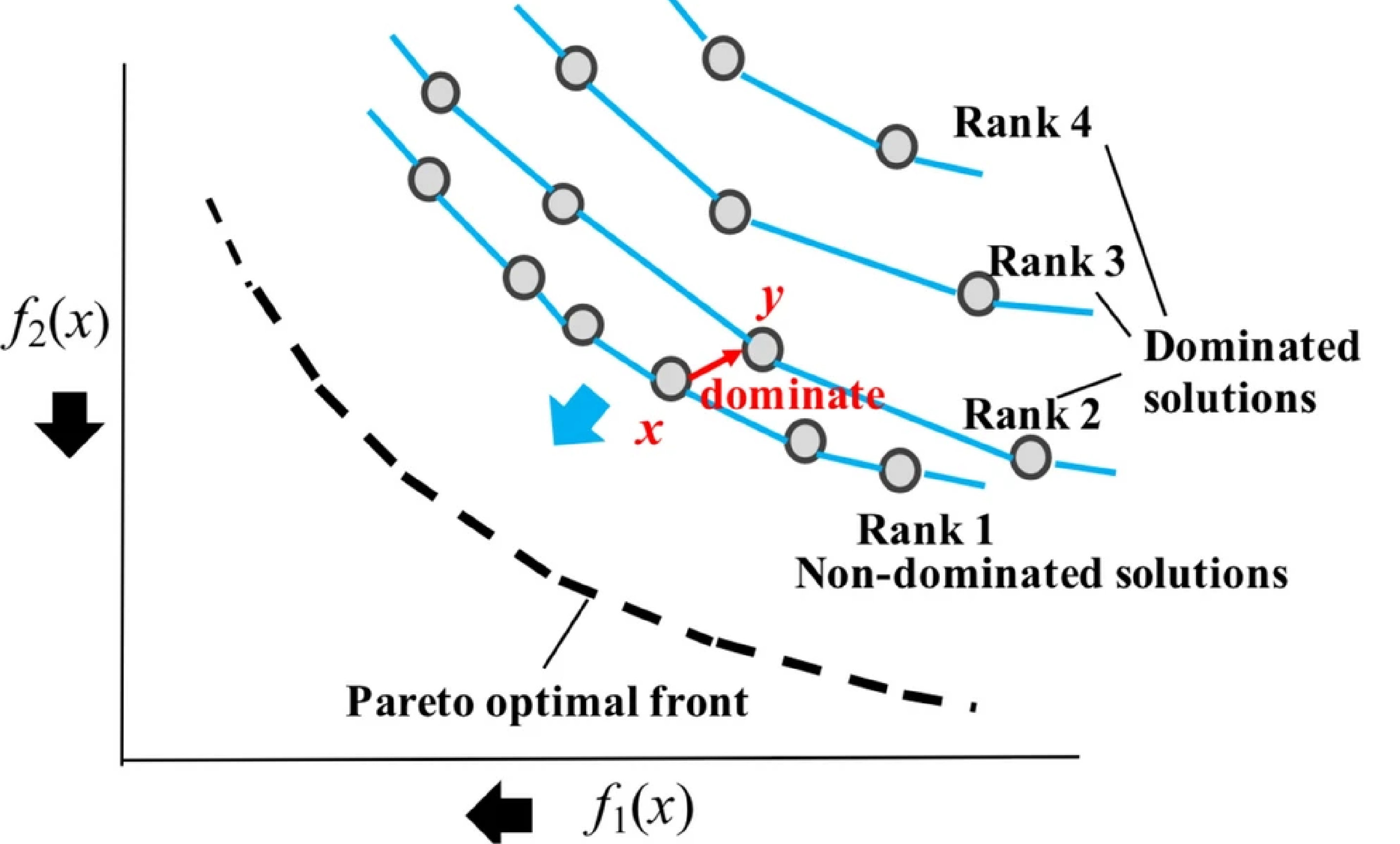Non-dominated levels illustration
  1. First Front: Contains all non-dominated solutions.
  2. Second Front: Non-dominated solutions after removing First Front solutions.
  3. Continue until all individuals are assigned to a front. Each individual is assigned a non-domination rank, with lower ranks indicating better solutions.
• Crowding Distance: When two solutions have the same non-domination rank, crowding distance measures solution density within its front. Solutions with larger crowding distances are preferred as they help maintain diversity and prevent premature convergence. Calculation method:
  1. Sort solutions within each front by each objective.
  2. Assign infinite crowding distance to boundary solutions (those with minimum and maximum objective values).
  3. For other solutions, crowding distance component for objective $m$ is $\frac{f_m(i+1) - f_m(i-1)}{f_m^{max} - f_m^{min}}$ for solution $i$.
  4. Total crowding distance is the sum across all objectives.

NSGA-II Algorithm Flow

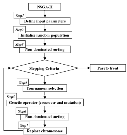NSGA-II algorithm flowchart

1. Initialize Population $P_0$: Generate random initial population of size $N$. Calculate objective values for each individual.

2. Non-dominated Sorting and Crowding Distance: Perform non-dominated sorting on current population $P_t$ (initially $P_0$) to get fronts $F_1, F_2, \dots$. Calculate crowding distance for individuals in each front.

3. Selection: Use binary tournament selection N times to select parent individuals. Each tournament compares two random individuals:
   • Prefer lower non-domination rank
   • If ranks equal, prefer larger crowding distance

4. Genetic Operators: Apply crossover and mutation to selected parents to create offspring population $Q_t$ of size $N$.

5. Combine Populations:
6. Elitism: Perform non-dominated sorting on combined population $R_t$. Select new parent population $P_{t+1}$ (size $N$):
   • Add entire fronts ($F_1, F_2, \dots$) until $P_{t+1}$ would exceed $N$.
   • For last front $F_k$, sort by crowding distance and add solutions until $P_{t+1}$ reaches size $N$.
7. Termination: Repeat steps 2-6 until termination criteria met (e.g., maximum generations, Pareto front stabilization).

NSGA-II Advantages

• Computational Efficiency: Fast non-dominated sorting with $O(M N^2)$ complexity ($M$ objectives, $N$ population size), better than NSGA’s $O(M N^3)$.
• Elitism: Preserves good solutions throughout evolution, improving convergence.
• Diversity Preservation: Effectively maintains population diversity through crowding distance, eliminating sharing parameter dependency.
• Wide Application: One of the most widely used algorithms in multi-objective optimization.

NSGA-II in pymoo

pymoo is a powerful Python framework for multi-objective optimization. It provides implementations of various algorithms including NSGA-II, and is easy to use and extend.

Using NSGA-II in pymoo typically involves:

1. Define Problem: Inherit from pymoo.core.problem.Problem and implement _evaluate method that takes decision variables x and returns objective values out['F'] (and optional constraint violations out['G']).

2. Select Algorithm: Import NSGA2 from pymoo.algorithms.moo.nsga2. Configure parameters like pop_size, crossover, and mutation operators.

3. Run Optimization: Use pymoo.optimize.minimize with problem instance, algorithm instance, termination criteria, and optional parameters (e.g., save_history, verbose).

4. Analyze Results: minimize returns a Result object containing non-dominated solutions (result.X for variables, result.F for objectives). Visualize Pareto front using pymoo.visualization tools.

pymoo Code Example

Here’s an example solving the classic ZDT1 bi-objective problem using NSGA-II in pymoo:

import numpy as np
from pymoo.algorithms.moo.nsga2 import NSGA2
from pymoo.problems.multi.zdt import ZDT1
from pymoo.operators.sampling.rnd import FloatRandomSampling
from pymoo.operators.crossover.sbx import SBXCrossover
from pymoo.operators.mutation.pm import PolynomialMutation
from pymoo.optimize import minimize
from pymoo.visualization.scatter import Scatter

# 1. Define problem
# ZDT1 is a built-in problem, we can use it directly.
# For custom problems, define like this:
# from pymoo.core.problem import Problem
# class MyProblem(Problem):
#     def __init__(self):
#         super().__init__(n_var=10, # number of decision variables
#                          n_obj=2,  # number of objectives
#                          n_constr=0, # number of constraints
#                          xl=0.0, # lower bound of variables
#                          xu=1.0) # upper bound of variables
#     def _evaluate(self, x, out, *args, **kwargs):
#         # x is a numpy array of shape (pop_size, n_var)
#         f1 = x[:, 0]
#         g = 1 + 9.0 / (self.n_var - 1) * np.sum(x[:, 1:], axis=1)
#         f2 = g * (1 - np.sqrt(f1 / g))
#         out["F"] = np.column_stack([f1, f2])
# problem = MyProblem()

problem = ZDT1(n_var=30) # ZDT1 problem has 30 decision variables

# 2. Select algorithm and configure parameters
algorithm = NSGA2(
    pop_size=100,      # population size
    n_offsprings=100,  # number of offspring per generation (usually equals pop_size)
    sampling=FloatRandomSampling(), # initial population sampling method
    crossover=SBXCrossover(prob=0.9, eta=15), # simulated binary crossover
    mutation=PolynomialMutation(eta=20),      # polynomial mutation
    eliminate_duplicates=True # eliminate duplicate individuals
)

# 3. Define termination criterion
from pymoo.termination import get_termination
termination = get_termination("n_gen", 400) # run for 400 generations

# 4. Run optimization
res = minimize(problem,
               algorithm,
               termination,
               seed=1, # set random seed for reproducibility
               save_history=True, # save optimization history
               verbose=True)     # print optimization progress

# 5. Results analysis and visualization
# Get Pareto front solutions
pareto_front_X = res.X # solutions in decision space
pareto_front_F = res.F # solutions in objective space

print("Number of Pareto optimal solutions found:", len(pareto_front_F))
# print("Pareto optimal solutions (objective space):\n", pareto_front_F)

# Visualize Pareto front
plot = Scatter(title="ZDT1 - Pareto Front (NSGA-II)")
plot.add(problem.pareto_front(), plot_type="line", color="black", alpha=0.7, label="True Pareto Front")
plot.add(pareto_front_F, color="red", s=30, label="Found Pareto Front")
plot.show()

# To view convergence process (requires matplotlib)
# try:
#     from pymoo.visualization.convergence import Convergence
#     conv = Convergence(res, problem=problem)
#     conv.plot()
#     conv.show()
# except ImportError:
#     print("matplotlib not installed. Skipping convergence plot.")

Code Explanation:

• ZDT1(n_var=30): Built-in test problem with two objectives and 30 decision variables.
• NSGA2(...): Creates NSGA-II instance:
  • pop_size: Population size.
  • n_offsprings: Number of offspring per generation.
  • sampling: Defines initial population generation.
  • crossover: Defines crossover operator. SBX is common for real-valued encoding.
  • mutation: Defines mutation operator.
  • eliminate_duplicates: Removes duplicates to maintain diversity.
• get_termination("n_gen", 400): Sets 400 generations as termination condition.
• minimize(...): Executes optimization:
  • Parameters include problem, algorithm, termination criteria
  • Options for saving history and printing progress
• Visualization: Uses Scatter to plot Pareto front.

Custom Problems and Operators

pymoo’s strength lies in its flexibility. You can easily define custom problems by inheriting from Problem and implementing _evaluate. You can also customize operators for specific problems.

Example custom problem:

from pymoo.core.problem import Problem
import numpy as np

class MyProblem(Problem):
    def __init__(self, n_var=2):
        # Define problem parameters: number of variables, objectives, constraints, variable bounds
        super().__init__(n_var=n_var,
                         n_obj=2,
                         n_constr=0, # Can set constraints with n_constr=1
                         xl=np.array([-5.0] * n_var),
                         xu=np.array([5.0] * n_var))

    def _evaluate(self, x, out, *args, **kwargs):
        # x is a numpy array of shape (pop_size, n_var)
        # Calculate objective function values
        f1 = np.sum((x - 1)**2, axis=1)
        f2 = np.sum((x + 1)**2, axis=1)

        out["F"] = np.column_stack([f1, f2])

        # If there are constraints, you can calculate and assign them like this:
        # g1 = x[:, 0]**2 + x[:, 1]**2 - 1  # Assume constraint is x1^2 + x2^2 <= 1
        # out["G"] = np.column_stack([g1])
```   # out["G"] = np.column_stack([g1])

Use this custom problem with NSGA-II as shown previously.

Summary

NSGA-II is an efficient and widely-used multi-objective optimization algorithm that balances convergence and diversity through non-dominated sorting and crowding distance calculations. The pymoo library provides convenient Python implementation for NSGA-II and other multi-objective optimization algorithms, allowing researchers and engineers to easily apply these algorithms to real-world problems. Through pymoo, you can readily define problems, configure algorithms, run optimizations, and analyze results.