Bootstrap resampling methods
Bootstrap Method
Core Idea and Basic Steps of Bootstrap
Bootstrap method, as its name suggests, draws inspiration from the absurd story of “pulling oneself up by one’s own bootstraps,” and was proposed by Efron in 1979. Its core idea is: when we only have one sample and know little about the population distribution, we treat this existing sample data (empirical distribution function, EDF) as the best approximation of the true population distribution. Then, by resampling with replacement from this “approximate population” to simulate the process of multiple independent sampling, we can estimate the properties of the estimator $ \hat{\theta} $ (such as sample mean, sample median, etc.) of the population parameter $ \theta $ (such as population mean, median, variance, etc.), including its sampling distribution, standard error, or confidence intervals.
This is a resampling method that involves independent sampling with replacement from existing sample data with the same sample size $ n $, and making inferences based on these resampled data.
Basic Steps 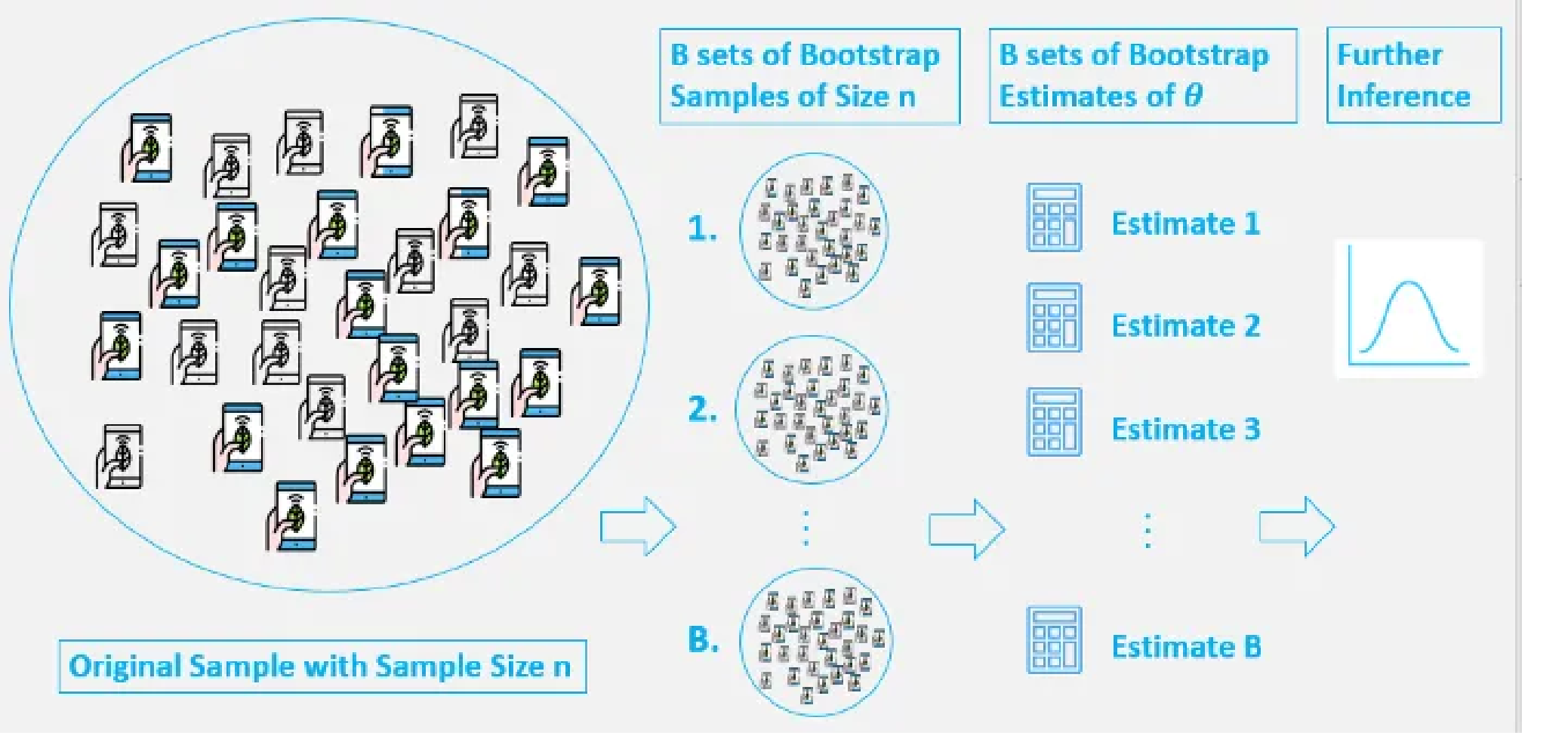
- Original Sample: We have an original sample $ S = {x_1, x_2, …, x_n} $ containing $ n $ observations drawn from an unknown population.
- Resampling with Replacement: Randomly draw $ n $ observations with replacement from the original sample $ S $ to form a new sample, called a Bootstrap Sample $ S^* $. Since sampling is done with replacement, some original observations may appear multiple times in $ S^* $, while others may not appear at all.
- Calculate Statistic: For each bootstrap sample $ S^* $, calculate the statistic $ \hat{\theta}^* $ of interest (e.g., mean, median, variance, correlation coefficient, etc.).
- Repeat: Repeat steps 2 and 3 a large number of times (e.g., B times, typically at least 1,000 or even 10,000 times for more stable results), obtaining B bootstrap statistics \(\hat{\theta}^*_1, \hat{\theta}^*_2, ..., \hat{\theta}^*_B\).
- Statistical Inference: Use these B Bootstrap statistics \(\{\hat{\theta}^*_1, ..., \hat{\theta}^*_B\}\) to construct an empirical sampling distribution. This distribution serves as an approximation of the true sampling distribution of \(\hat{\theta}\). Based on this distribution, we can:
- Estimate the standard error (SE) of the statistic $ \hat{\theta} $.
- Construct confidence intervals (CI) for the statistic $ \hat{\theta} $.
- Perform hypothesis testing.
Core Analogy: “Sub-sample is to sample, as sample is to population.” The brilliance of Bootstrap lies in using the variability of resampling from the sample to model the variability of sampling from the population.
Original Motivation and Objectives of Bootstrap
- Standard Error Estimation: The standard errors of many statistics are analytically difficult to derive, especially for complex statistics (such as medians, quantiles, correlation coefficients, and certain non-standard estimates of regression coefficients). Bootstrap provides a general, simulation-based numerical computation method.
- Confidence Interval Construction: When the underlying distribution of the data is unknown or does not conform to the normality assumptions of classical statistical methods (such as t-tests, Z-tests), or when the sample size is small, Bootstrap can construct more reliable confidence intervals.
- Hypothesis Testing: Although not as commonly used as the previous two, the Bootstrap concept can also be used to construct non-parametric hypothesis tests.
- Reduced Dependence on Distribution Assumptions: As a non-parametric or semi-parametric method (depending on specific implementation), Bootstrap relaxes strict requirements on the form of the population distribution.
- Handling Small Sample Problems: Traditional methods that rely on large sample theory may fail with small samples; Bootstrap provides an alternative.
- Evaluating Model Stability and Prediction Uncertainty: In machine learning, techniques like Bagging (Bootstrap Aggregating) utilize Bootstrap to improve model stability and accuracy.
Types of Bootstrap
Non-parametric Bootstrap
This is the most common form of Bootstrap, with the process as described in the basic steps. It does not assume a specific form for the population distribution, but instead resamples directly from the empirical distribution function (EDF) of the original sample.
Bootstrap Estimation of Standard Error of an Estimator: Let \(\hat{\theta}\) be an estimator of parameter \(\theta\) calculated based on the original sample \(x_1, ..., x_n\). We generate B Bootstrap samples and calculate the corresponding Bootstrap estimates \(\hat{\theta}_1^*, \hat{\theta}_2^*, ..., \hat{\theta}_B^*\) for each sample. The Bootstrap estimate of the standard error \(\hat{SE}_{boot}(\hat{\theta})\) can be calculated as the standard deviation of these Bootstrap estimates:
\[\begin{equation} \hat{SE}_{boot}(\hat{\theta}) = \sqrt{\frac{1}{B-1} \sum_{i=1}^B (\hat{\theta}_i^* - \bar{\theta}^*)^2} \end{equation}\]where $ \bar{\theta}^* = \frac{1}{B} \sum_{i=1}^B \hat{\theta}_i^* $ is the mean of the Bootstrap estimates.
Bootstrap Estimation of Mean Squared Error (MSE) of an Estimator: If we are concerned with the mean squared error of estimator $ \hat{\theta} $ relative to the true parameter $ \theta $, $ MSE_F(\hat{\theta}) = E_F[(\hat{\theta} - \theta)^2] $, Bootstrap can provide an approximate estimate. A common method is to estimate $ E_{F_n}[(\hat{\theta}^* - \hat{\theta})^2] $, namely:
\[\begin{equation} \hat{MSE}_{boot} = \frac{1}{B} \sum_{i=1}^B (\hat{\theta}_i^* - \hat{\theta})^2 \end{equation}\]where $ \hat{\theta} $ is the estimate from the original sample. This actually estimates an approximation of variance plus squared bias.
Bootstrap Confidence Intervals (Percentile Method): This is one of the most direct methods for constructing confidence intervals.
- Obtain B Bootstrap estimates \(\hat{\theta}_1^*, \hat{\theta}_2^*, ..., \hat{\theta}_B^*\).
- Sort these estimates in ascending order: \(\hat{\theta}_{(1)}^* \le \hat{\theta}_{(2)}^* \le ... \le \hat{\theta}_{(B)}^*\).
- For a confidence level of $ 1-\alpha $, find the $ k_1 = \lfloor B \times (\alpha/2) \rfloor $ th value and the $ k_2 = \lceil B \times (1-\alpha/2) \rceil $ th value (or more simply, take the $ B \times (\alpha/2) $ and $ B \times (1-\alpha/2) $ percentiles).
- Then \((\hat{\theta}_{(k_1)}^*, \hat{\theta}_{(k_2)}^*)\) is the $ 1-\alpha $ Bootstrap percentile confidence interval for \(\theta\). For example, for a 95% confidence interval (\(\alpha = 0.05\)), we would take the 2.5th percentile and the 97.5th percentile.
Parametric Bootstrap
When we can make assumptions about the form of the population distribution function $ F(x; \beta) $, but the parameters $ \beta $ (which can be a vector) are unknown, we can use parametric Bootstrap.
The steps are as follows:
- Parameter Estimation: Use the original sample $ X_1, X_2, …, X_n $ to estimate the unknown parameters $ \beta $, obtaining the estimate $ \hat{\beta} $ (for example, through maximum likelihood estimation).
- Generate Parametric Bootstrap Samples: Generate B new samples of size \(n\) from the fitted parametric distribution \(F(x; \hat{\beta})\). Each such sample \(X_1^*, ..., X_n^*\) is randomly drawn from \(F(x; \hat{\beta})\).
- Calculate Statistics: Calculate the statistic of interest $ \hat{\theta}^* $ for each parametric Bootstrap sample.
- Statistical Inference: Use these B $ \hat{\theta}^* $ to construct an empirical sampling distribution; subsequent steps are similar to non-parametric Bootstrap (calculating standard error, confidence intervals, etc.).
The effectiveness of parametric Bootstrap depends on how well the chosen parametric model $ F(x; \beta) $ fits the true data-generating process. If the model is not chosen appropriately, the results may be biased.
Differences Between Bootstrap and Mark-Recapture Methods
| Feature | Bootstrap | Mark-Recapture |
|---|---|---|
| Main Purpose | Estimating sampling distributions, standard errors, confidence intervals of any statistic. | Primarily used in ecology to estimate the size of closed populations (Population Size Estimation). |
| Data Source | Based on an already obtained sample data. | Based on at least two actual captures and observations of the real population. |
| Meaning of “Resampling” | Resampling with replacement from the original sample to generate bootstrap samples (computer simulation). | Refers to repeated capture events of the population, observing the proportion of marked individuals (actual field operation). |
| Application Fields | Widely used in statistics, machine learning, econometrics, etc. | Mainly in ecology and wildlife management. |
Differences Between Bootstrap and Monte Carlo Methods
Monte Carlo methods are a broader category of computational techniques that rely on repeated random sampling to obtain numerical results. Bootstrap can be viewed as a specific application of Monte Carlo methods, with its distinguishing feature being sampling from the empirical distribution function (EDF) of the data.
| Feature | Bootstrap | Monte Carlo Methods (General) |
|---|---|---|
| Core Idea | Sampling with replacement from the empirical distribution function (EDF) of observed data. | Obtaining numerical approximations based on a large number of random samples and statistical trials. |
| Data Generation Source | Based on existing sample data with replacement (replicating data from the original sample). Heavily depends on the quality and representativeness of the original sample. | Usually generates new data from a known or assumed theoretical probability distribution (e.g., normal, uniform). Doesn’t require original data, only distribution assumptions. |
| Main Purpose | Statistical inference: estimating properties of statistics (standard errors, confidence intervals). | More general: numerical integration, complex system simulation, optimization, posterior sampling in Bayesian inference, etc. |
| Population Assumptions | The original sample is a good representation of the population. | Can directly simulate a known population distribution, or explore systems described by random processes. |
Comparison of Application Scenarios:
| Problem Type | Monte Carlo Simulation (General) | Bootstrap |
|---|---|---|
| Known Theoretical Distribution | ✔️ Directly generates data from theoretical distribution. | ❌ (Non-parametric Bootstrap doesn’t rely on theoretical distribution assumptions) / ✔️ (Parametric Bootstrap based on fitted theoretical distribution) |
| Unknown Distribution (only sample available) | ❌ (Unless first fitting a distribution to the sample then simulating) | ✔️ Directly resamples from the empirical distribution of the sample. |
| High-dimensional Integration | ✔️ (Common method, e.g., importance sampling) | ❌ (Not primarily used for this) |
| Confidence Intervals for Statistics | ❓ (Possible if distribution of statistic is known, otherwise difficult) | ✔️ One of its main applications, can estimate without distribution assumptions. |
| Small Sample Problems | ❓ (Depends on accuracy of distribution assumptions) | ✔️ “Amplifies” sample information through resampling, commonly used for small sample inference. |
Python Implementation
Manual Implementation Using numpy
1
2
3
4
5
6
7
8
9
10
11
12
13
14
15
16
17
18
19
20
21
22
23
24
25
26
27
28
29
30
31
import numpy as np

def bootstrap_statistic_manual(data, statistic_func, n_iterations=1000):
    """
    Manually performs the Bootstrap process to estimate the distribution of a statistic.
    """
    n_size = len(data)
    bootstrap_stats = []
    for _ in range(n_iterations):
        bootstrap_sample = np.random.choice(data, size=n_size, replace=True)
        stat = statistic_func(bootstrap_sample)
        bootstrap_stats.append(stat)
    return bootstrap_stats

# Example data
original_sample = np.array([2, 3, 5, 7, 11, 13, 17, 19, 23, 29, 5, 8, 10])
print(f"Original sample: {original_sample}")
original_mean = np.mean(original_sample)
print(f"Original sample mean: {original_mean:.2f}")

# Manual Bootstrap for mean
bootstrap_means_manual = bootstrap_statistic_manual(original_sample, np.mean, n_iterations=10000)
std_error_mean_manual = np.std(bootstrap_means_manual, ddof=1)
# Percentile confidence interval
alpha = 0.05
lower_manual = np.percentile(bootstrap_means_manual, 100 * (alpha / 2))
upper_manual = np.percentile(bootstrap_means_manual, 100 * (1 - alpha / 2))

print(f"\n--- Manual Numpy Implementation (Mean) ---")
print(f"Bootstrap estimated standard error: {std_error_mean_manual:.2f}")
print(f"95% percentile confidence interval: [{lower_manual:.2f}, {upper_manual:.2f}]")
Using scipy.stats.bootstrap
scipy provides the scipy.stats.bootstrap function, which makes Bootstrap analysis very convenient.
scipy.stats.bootstrap(data, statistic, *, n_resamples=9999, confidence_level=0.95, method='BCa', random_state=None, axis=0, batch=None)
Main parameter descriptions:
data: One or more sample data sequences. For a single sample, it can be a one-dimensional array. For multiple samples (e.g., for comparing differences in statistics between two independent samples), it can be a tuple or list containing multiple one-dimensional arrays.statistic: A callable object (function) that takesdata(or samples drawn fromdata) as a parameter and returns the calculated statistic. The function must be able to handle theaxisparameter (ifdatais multidimensional or used for multi-sample situations).n_resamples: Number of Bootstrap resamples. Default is 9999.confidence_level: Confidence level for the confidence interval. Default is 0.95 (i.e., 95% confidence interval).method: Method for calculating confidence intervals. Common options include:'percentile': Percentile method (what we manually implemented earlier).'basic': Basic Bootstrap method (also known as the pivot method).'BCa': Bias-Corrected and accelerated Bootstrap method. This is generally considered more accurate, especially for biased statistics or asymmetric distributions, and is the default method inscipy.
random_state: Used to control reproducibility of random number generation. Can be an integer or anp.random.Generatorinstance.axis: Ifdatais a multidimensional array, specifies along which axis to calculate the statistic.batch: If provided, performs resampling in batch mode, which can save memory but may be slightly slower.
Return value: A BootstrapResult object containing the following main attributes:
confidence_interval: AConfidenceIntervalobject withlowandhighattributes, representing the lower and upper bounds of the confidence interval.standard_error: Bootstrap estimated standard error.bootstrap_distribution: (Optional, ifmethodsupports andbatchis not used) Array of all Bootstrap statistics.
Example code:
1
2
3
4
5
6
7
8
9
10
11
12
13
14
15
16
17
18
19
20
21
22
23
24
25
26
27
28
29
30
31
32
33
34
35
36
37
38
39
40
41
42
43
44
45
46
47
48
from scipy import stats
import numpy as np

# Example data
original_sample = np.array([2, 3, 5, 7, 11, 13, 17, 19, 23, 29, 5, 8, 10])
n_resamples = 10000 # Consistent with manual implementation

print(f"\n--- Scipy Implementation (Mean) ---")
# For single sample statistics, the statistic function usually receives one sample
# data needs to be in the form of (sample,) or a list/tuple containing a single sample
# scipy.stats.bootstrap expects data to be a sequence of sequences, even if there's only one sample
data_for_scipy = (original_sample,)

# Estimate confidence interval and standard error for the mean
# Using BCa method (default)
res_mean_bca = stats.bootstrap(data_for_scipy, np.mean, n_resamples=n_resamples, random_state=42)
print(f"BCa method 95% confidence interval (mean): [{res_mean_bca.confidence_interval.low:.2f}, {res_mean_bca.confidence_interval.high:.2f}]")
print(f"BCa method estimated standard error (mean): {res_mean_bca.standard_error:.2f}")

# Using percentile method
res_mean_percentile = stats.bootstrap(data_for_scipy, np.mean, method='percentile', n_resamples=n_resamples, random_state=42)
print(f"Percentile method 95% confidence interval (mean): [{res_mean_percentile.confidence_interval.low:.2f}, {res_mean_percentile.confidence_interval.high:.2f}]")
print(f"Percentile method estimated standard error (mean): {res_mean_percentile.standard_error:.2f}")


print(f"\n--- Scipy Implementation (Median) ---")
# Estimate confidence interval and standard error for the median
res_median_bca = stats.bootstrap(data_for_scipy, np.median, n_resamples=n_resamples, random_state=42)
print(f"BCa method 95% confidence interval (median): [{res_median_bca.confidence_interval.low:.2f}, {res_median_bca.confidence_interval.high:.2f}]")
print(f"BCa method estimated standard error (median): {res_median_bca.standard_error:.2f}")

res_median_percentile = stats.bootstrap(data_for_scipy, np.median, method='percentile', n_resamples=n_resamples, random_state=42)
print(f"Percentile method 95% confidence interval (median): [{res_median_percentile.confidence_interval.low:.2f}, {res_median_percentile.confidence_interval.high:.2f}]")
print(f"Percentile method estimated standard error (median): {res_median_percentile.standard_error:.2f}")

# Example: Comparing the difference in means between two independent samples
sample1 = np.array([1, 2, 3, 4, 5, 6])
sample2 = np.array([3, 5, 7, 9])

def diff_means(s1, s2, axis=0): # statistic function needs to handle axis for multi-sample input
    return np.mean(s1, axis=axis) - np.mean(s2, axis=axis)

data_two_samples = (sample1, sample2)
res_diff_means = stats.bootstrap(data_two_samples, diff_means, n_resamples=n_resamples, random_state=42)
print(f"\n--- Scipy Implementation (Difference in Means of Two Independent Samples) ---")
print(f"Original samples mean difference: {np.mean(sample1) - np.mean(sample2):.2f}")
print(f"BCa method 95% confidence interval (mean difference): [{res_diff_means.confidence_interval.low:.2f}, {res_diff_means.confidence_interval.high:.2f}]")
print(f"BCa method estimated standard error (mean difference): {res_diff_means.standard_error:.2f}")
Notes:
- When passing a single sample to
stats.bootstrap, thedataparameter typically expects a tuple or list containing that sample, such as(original_sample,)or[original_sample]. This is because the function is designed to handle multiple samples (e.g., comparing mean differences between two samples). - The function passed to
statisticshould be able to accept operations along the axis specified by theaxisparameter, especially when handling multidimensional data or multi-sample situations. For NumPy functions likenp.mean,np.median, etc., they already support theaxisparameter.
Applications, Advantages, and Limitations of Bootstrap
Bootstrap has very wide applications, including:
- Estimating standard errors and confidence intervals for means, medians, variances, correlation coefficients, regression coefficients, etc.
- Comparing differences between two or more groups in A/B testing, especially when data distributions are irregular or sample sizes are small.
- Bagging in machine learning (e.g., Random Forests), stability assessment of model parameters.
- Estimating Value at Risk (VaR) and Expected Shortfall in finance.
- Assessing confidence in phylogenetic trees in bioinformatics.
Advantages:
- Versatility: Can be applied to various statistics, including those without simple analytical expressions for standard errors or sampling distributions (such as medians, percentiles, Kendall’s tau, etc.).
- Reduced Distribution Assumptions: Non-parametric Bootstrap makes very few assumptions about the population distribution, only requiring that the samples are independently and identically distributed.
- Conceptually Simple, Easy to Implement: The basic idea is intuitive, and programming implementation is relatively easy.
- Handles Complex Estimators: For complex model parameters or statistics, Bootstrap is often one of the few feasible inference methods.
- Generally Performs Well: In many situations, especially with sufficiently large original samples, Bootstrap provides fairly accurate standard errors and confidence intervals.
Limitations:
- Computationally Intensive: Requires a large number of repeated samplings and calculations, which can be time-consuming for very large datasets or complex statistical calculations.
- Dependent on Original Sample Quality: Bootstrap results are highly dependent on how representative the original sample is of the population. If the original sample is biased or contains outliers, Bootstrap results may also be affected. “Garbage in, garbage out.”
- Small Sample Issues: Although commonly used for small samples, if the original sample is too small, its empirical distribution may not well represent the population distribution, leading to unstable or biased Bootstrap results.
- May Not Perform Well for Extreme Values: For statistics that depend on information from the tails of the data distribution (e.g., extreme values), Bootstrap may not perform well.
- Potentially Overoptimistic: Sometimes, especially in small sample situations, Bootstrap confidence intervals may be narrower than the true confidence intervals (i.e., overly optimistic).
- Not Universal: For certain problems, such as estimating bounds of population parameters (like the maximum of a uniform distribution), standard Bootstrap may fail. Specific variants or adjustments are needed.
- Choice of Bootstrap Method: There are multiple methods for constructing Bootstrap confidence intervals (Percentile, Basic, BCa, Studentized Bootstrap), which perform differently in various situations. BCa is generally considered a better choice, but its computation is also more complex.
Summary
Bootstrap is a powerful and flexible statistical tool that, through the power of computer simulation, allows us to make inferences about the properties of various statistics without making too many parametric assumptions about the data. It plays an increasingly important role in modern statistics and data science. Understanding its principles, applicable scenarios, and potential limitations is crucial for correctly and effectively applying it. The emergence of libraries like scipy has made the application of Bootstrap more convenient.